Bayesian Analysis of Aviation Accidents

Introduction

This project models the fatality rates of airplane crashes from 1975 to 2024. We use non-hierarchical and hierarchical Bayesian models with the airplane manufacturer as the grouping variable in the hierarchical model. Specifically, we compare two non-hierarchical models (complete pooling and no pooling) against one hierarchical model (partial pooling).

Motivation

Aviation has undergone massive developments since the first commercial flight in 1914. Airplane safety has always been the top priority for airlines; a single airplane crash will drive away customers to safer perceived airlines and, of course, cost lives. Although this priority of making airplanes as safe as possible has significantly reduced the number of crashes over the years, accidents still continue to occur.

Not all accidents are the same; survivability in crashes varies significantly. Understanding which factors influence survivability in crashes remains crucial for manufacturers and airlines seeking to minimize the loss of life. While accident prevention remains the most important priority, understanding the fatality patterns when accidents do occur is equally important in discussions of airplane safety.

Problem

When aviation accidents occur, the fatality rates vary significantly — from incidents where all passengers survive to catastrophic losses of everyone on board. This variation raises critical questions: Has the likelihood of surviving an airplane crash improved over time? Do certain airplane manufacturers demonstrate consistently higher crash survival rates than others? How much of the variation in crash fatality rates can be attributed to crash-specific details of individual accidents versus inherent airplane characteristics? These are questions that we hope to answer in our report.

Main Modeling Idea

We address these questions using hierarchical and non-hierarchical Bayesian modeling of fatality rates across aviation accidents from 1975 to 2024. We assume that aircraft from the same manufacturer share some of the same characteristics, such as similar design choices, engineering approaches, and safety systems. We still account for the overall similarity between all aircraft by including a global population-level distribution. We compare a partial pooling model against two baselines: complete pooling and no pooling.

Dataset

The dataset was obtained from a Kaggle repository created by Jonathan Ogwumike [1]. According to the repository description, the dataset has been used to teach students about Power BI and Python.

The dataset has two notable projects linked to it. Both are written in Python, and neither uses hierarchical models to analyze the fatality rate trend. Both include some exploratory data analysis, but since these are in Python we wrote our own analysis code in R.

Data Description

Crashes Over Time

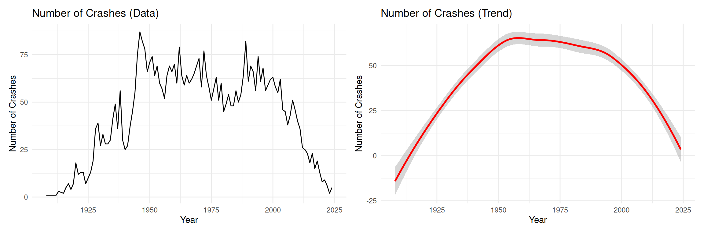
# Figure 1: Number of crashes - data
fig1 <- crashes %>%
  group_by(year) %>%
  summarise(n_crashes = n()) %>%
  ggplot(aes(x = year, y = n_crashes)) +
  geom_line() +
  labs(title = "Number of Crashes (Data)",
       x = "Year", y = "Number of Crashes")

# Figure 2: Number of crashes - trend
fig2 <- crashes %>%
  group_by(year) %>%
  summarise(n_crashes = n()) %>%
  ggplot(aes(x = year, y = n_crashes)) +
  geom_smooth(method = "loess", color = "red", se = TRUE) +
  labs(title = "Number of Crashes (Trend)",
       x = "Year", y = "Number of Crashes")

fig1 + fig2

Temporal trends in aviation accidents

Fatalities Over Time

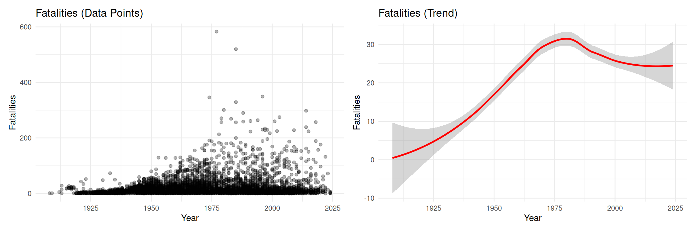
# Figure 3: Fatalities - data points
fig3 <- crashes %>%
  ggplot(aes(x = year, y = fatalities)) +
  geom_point(alpha = 0.3) +
  labs(title = "Fatalities (Data Points)",
       x = "Year", y = "Fatalities")

# Figure 4: Fatalities - trend
fig4 <- crashes %>%
  ggplot(aes(x = year, y = fatalities)) +
  geom_smooth(method = "loess", color = "red", se = TRUE) +
  labs(title = "Fatalities (Trend)",
       x = "Year", y = "Fatalities")

fig3 + fig4

Trends in aviation accidents

Fatality Rate Over Time

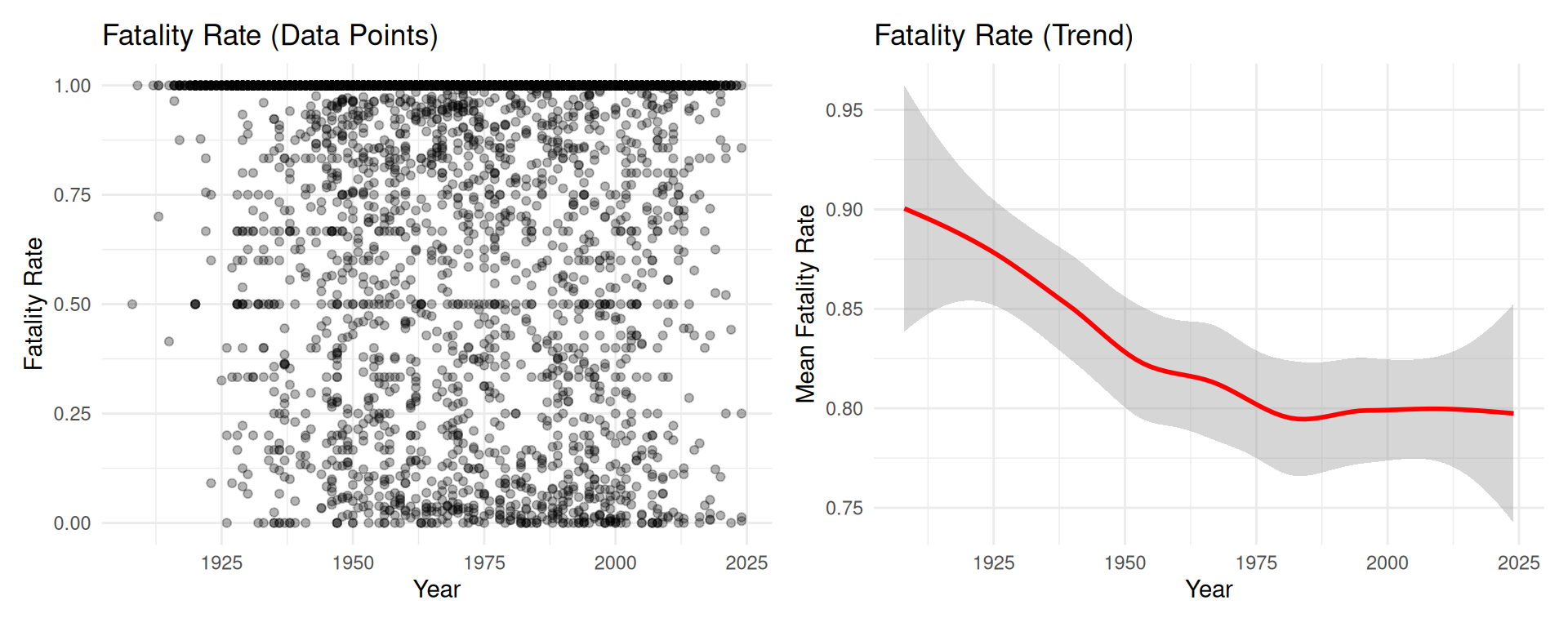
# Compute yearly mean fatality rate
rate_ts <- crashes %>%
  group_by(year) %>%
  summarise(
    mean_rate = mean(fatality_rate, na.rm = TRUE),
    sd_rate = sd(fatality_rate, na.rm = TRUE),
    n = n(),
    se = ifelse(n > 1, sd_rate / sqrt(n), NA_real_)
  )

# Figure 5: Fatality rate - data points
fig5 <- crashes %>%
  ggplot(aes(x = year, y = fatality_rate)) +
  geom_point(alpha = 0.3) +
  labs(title = "Fatality Rate (Data Points)",
       x = "Year", y = "Fatality Rate")

# Figure 6: Fatality rate - trend
fig6 <- ggplot(rate_ts, aes(x = year, y = mean_rate)) +
  geom_smooth(method = "loess", color = "red", se = TRUE) +
  labs(title = "Fatality Rate (Trend)",
       x = "Year", y = "Mean Fatality Rate")

fig5 + fig6

Mean fatality rate by year

To conduct a modern analysis on plane crash fatalities, we do not want to include observations from far back in the history. We need some reasonable cutoff point that keeps sufficient amount of data and allows us to model modern aircraft data. The fatalities trend shows a turning point around 1975, so it is reasonable to choose that as our observation cutoff year. This filtering brings our total observation count from 5013 down to 2188, so we are still left with plenty of data. We also only include observations from manufacturers with at least 10 crashes present in the data to stabilize the no pooling and partial pooling models. This brought our data down to 1766 observations.

1975 is a good cutoff date, because it resembles a period that shares lots of characteristics with modern flight travel. The 1950s and 1960s saw an upsurge in commercial flights, aircraft carriers, and international flying routes [2]. This upsurge was accompanied by great technological innovations. The most notable ones were the jet engine in the 1950s (safer and more reliable than the earlier piston engines) and the introduction of electronic instruments to the cockpit in the 1970s [3].

len_before <- nrow(crashes)
crashes_filtered <- crashes %>% filter(year > 1975)
len_after <- nrow(crashes_filtered)

cat("Observations before filtering:", len_before, "\n")

Observations before filtering: 5013 

cat("Observations after filtering:", len_after, "\n")

Observations after filtering: 2188 

cat("Rows removed:", len_before - len_after, "\n")

Rows removed: 2825 

len_before <- nrow(crashes_filtered)
n_manufacturers_before <- n_distinct(crashes_filtered$aircraft_manufacturer)

min_crashes <- 10
crashes_filtered <- crashes_filtered %>%
  group_by(aircraft_manufacturer) %>%
  filter(n() >= min_crashes) %>%
  ungroup()

len_after <- nrow(crashes_filtered)
n_manufacturers_after <- n_distinct(crashes_filtered$aircraft_manufacturer)

cat("Observations before filtering:", len_before, "\n")

Observations before filtering: 2188 

cat("Observations after filtering:", len_after, "\n")

Observations after filtering: 1766 

cat("Rows removed:", len_before - len_after, "\n")

Rows removed: 422 

cat("Manufacturers before filtering:", n_manufacturers_before, "\n")

Manufacturers before filtering: 304 

cat("Manufacturers after filtering:", n_manufacturers_after, "\n")

Manufacturers after filtering: 40 

crashes_filtered %>%
  select(where(is.numeric)) %>%
  skim()

Data summary

Name	Piped data
Number of rows	1766
Number of columns	7
_______________________
Column type frequency:
numeric	7
________________________
Group variables	None

Variable type: numeric

skim_variable	n_missing	complete_rate	mean	sd	p0	p25	p50	p75	p100	hist
year	0	1	1994.59	11.41	1976.0	1986.00	1994.00	2003.00	2024.00	▆▇▆▅▁
day	0	1	15.96	8.73	1.0	9.00	16.00	24.00	31.00	▇▇▇▇▆
ground	0	1	3.89	92.80	0.0	0.00	0.00	0.00	2750.00	▇▁▁▁▁
fatalities	0	1	29.57	48.77	0.0	4.00	11.00	32.00	583.00	▇▁▁▁▁
aboard	0	1	45.07	64.65	1.0	8.00	18.00	52.00	644.00	▇▁▁▁▁
fatality_rate	0	1	0.78	0.34	0.0	0.64	1.00	1.00	1.00	▂▁▁▁▇
year_scaled	0	1	0.95	0.46	0.2	0.60	0.92	1.29	2.13	▆▇▆▅▁

Empirical Fatality Rates by Manufacturer

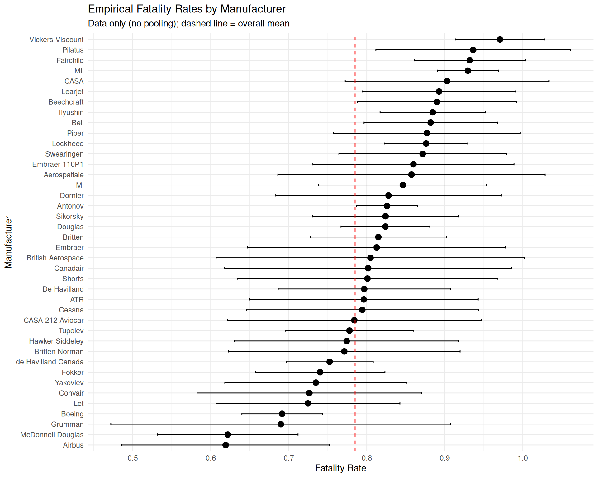
# Compute empirical fatality rates by manufacturer (≥10 crashes)
empirical_rates <- crashes_filtered %>%
  group_by(aircraft_manufacturer) %>%
  summarise(
    mean_rate = mean(fatality_rate, na.rm = TRUE),
    sd_rate = sd(fatality_rate, na.rm = TRUE),
    n = n(),
    se = ifelse(n > 1, sd_rate / sqrt(n), NA_real_),
    .groups = "drop"
  ) %>%
  mutate(
    lower_ci = mean_rate - 1.96 * se,
    upper_ci = mean_rate + 1.96 * se
  ) %>%
  arrange(mean_rate)

# Plot empirical rates
empirical_rates %>%
  mutate(aircraft_manufacturer = fct_reorder(aircraft_manufacturer, mean_rate)) %>%
  ggplot(aes(x = mean_rate, y = aircraft_manufacturer)) +
  geom_point(size = 3) +
  geom_errorbarh(aes(xmin = lower_ci, xmax = upper_ci), height = 0.2) +
  geom_vline(
    xintercept = mean(crashes_filtered$fatality_rate), 
    linetype = "dashed", 
    color = "red"
  ) +
  labs(
    title = "Empirical Fatality Rates by Manufacturer",
    subtitle = "Data only (no pooling); dashed line = overall mean",
    x = "Fatality Rate", 
    y = "Manufacturer"
  ) +
  theme_minimal()

Data Modeling

We model airplane crash fatality rates using three Bayesian models, each making different assumptions about information sharing across manufacturers. All models treat the number of fatalities \(y_i\) in crash \(i\) as binomially distributed given the number of people aboard \(n_i\) and a crash-specific fatality probability \(p_i\).

We use the logit link to constrain all predictions to \([0, 1]\):

\[\operatorname{logit}(p_i) = \ln\!\left(\frac{p_i}{1-p_i}\right)\]

When \(\eta_i\) is a linear predictor, solving for \(p_i\) gives:

\[p_i = \frac{\exp(\eta_i)}{1 + \exp(\eta_i)}\]

This allows linear predictors \(\eta_i \in (-\infty, \infty)\) to produce valid fatality probabilities.

Complete Pooling (Non-Hierarchical)

A complete pooling model assumes all observations are drawn from a single global distribution. In our plane crash setting this means every crash follows the same distribution regardless of manufacturer or any other grouping:

\[\begin{align*} y_i &\sim \text{Binomial}(n_i, p_i) \\ \text{logit}(p_i) &= \alpha + \beta \cdot \text{year\_scaled}_i \end{align*}\]

The strength of this model is its simplicity; its weakness is that it cannot capture manufacturer-level differences.

No Pooling (Non-Hierarchical)

A no pooling model gives each manufacturer its own completely independent distribution, with no information shared across groups. With \(m[i]\) denoting the manufacturer of crash \(i\):

\[\begin{align*} y_i &\sim \text{Binomial}(n_i, p_i) \\ \text{logit}(p_i) &= \alpha_{m[i]} + \beta_{m[i]} \cdot \text{year\_scaled}_i \end{align*}\]

This captures manufacturer-level differences but risks overfitting for manufacturers with few crashes, since they cannot borrow information from others.

Partial Pooling (Hierarchical)

A partial pooling model combines both approaches: each manufacturer has its own parameters, but those parameters are drawn from a shared global distribution. This regularizes estimates for manufacturers with little data by pulling them toward the global mean:

\[\begin{align*} y_i &\sim \text{Binomial}(n_i, p_i) \\ \text{logit}(p_i) &= \alpha_0 + \beta_0 \cdot \text{year\_scaled}_i + \alpha_{m[i]} + \beta_{m[i]} \cdot \text{year\_scaled}_i \\[0.5em] \begin{bmatrix} \alpha_m \\ \beta_m \end{bmatrix} &\sim \mathcal{N}\!\left(\begin{bmatrix} 0 \\ 0 \end{bmatrix},\, \boldsymbol{\Sigma}\right), \quad \boldsymbol{\Sigma} = \begin{bmatrix} \sigma_\alpha^2 & \rho\,\sigma_\alpha\sigma_\beta \\ \rho\,\sigma_\alpha\sigma_\beta & \sigma_\beta^2 \end{bmatrix} \end{align*}\]

The manufacturer-level effects \(\alpha_m\) and \(\beta_m\) are drawn from a multivariate normal distribution, which solves the overfitting problem of no pooling by borrowing strength from the global distribution.

Prior Selection

Global Intercept

For the global intercept \(\alpha\), we use a weakly informative prior centered on the observed fatality rate of \(\approx 0.8\), transformed to the logit scale:

\[\operatorname{logit}(0.8) = \ln\!\left(\frac{0.8}{0.2}\right) \approx 1.386 \approx 1.4\]

We use \(\alpha \sim \mathcal{N}(1.4,\, 1)\). The standard deviation of 1 keeps the prior weakly informative without over-constraining the estimate.

Global Year Coefficient

For the year coefficient \(\beta\), we use a more conservative prior. The fatality rate plot shows only a slight yearly trend, so we use \(\beta \sim \mathcal{N}(0,\, 0.5)\), yielding a 95% credible interval of approximately \([-1.0,\, 1.0]\).

Manufacturer-Level Priors (No Pooling)

For the manufacturer-specific intercepts and slopes in the no pooling model, we use \(\mathcal{N}(0,\, 1)\) — a safe, weakly informative choice that allows the data to dominate while keeping estimates in a reasonable range. brms requires a single prior class for all manufacturer-level coefficients, making it impractical to set manufacturer-specific priors.

Group-Level Standard Deviation (Partial Pooling)

For the group-level standard deviation \(\sigma\) in the hierarchical model, we observe that manufacturer fatality rates fall roughly between 0.6 and 0.95 across all manufacturers. Assuming this range covers \(\pm 2\sigma\) on the logit scale:

\[\sigma \approx \frac{\operatorname{logit}(0.95) - \operatorname{logit}(0.6)}{4} \approx 0.635\]

We use a half-normal prior \(\sigma \sim \mathcal{N}^+(0,\, 0.6)\), whose expected value is \(E[X] = 0.6\sqrt{2/\pi} \approx 0.479\).

Correlation Coefficient \(\rho\)

For the correlation \(\rho\) between manufacturer-level intercepts and slopes, we use \(\rho \sim \text{LKJ}(2)\). The LKJ distribution is designed for correlation matrices. With shape parameter \(\eta = 2 > 1\), the prior is skeptical of extreme correlations, producing a bell-shaped distribution centered at zero.

Complete pooling (non-hierarchical model)

Complete Pooling Model

With \(i\) representing individual crashes, \(n_i\) representing the number of people aboard, and \(p_i\) representing the fatality probability of a crash, the model is:

\[\begin{align*} \text{Likelihood:} \quad & \\ y_i &\sim \text{Binomial}(n_i, p_i) \\ \text{logit}(p_i) &= \alpha + \beta \cdot \text{year\_scaled}_i \\[1em] \text{Priors:} \quad & \\ \alpha &\sim \mathcal{N}(1.4,\, 1) \\ \beta &\sim \mathcal{N}(0,\, 0.5) \end{align*}\]

The complete pooling model is the simplest of our three models. The model assumes that each manufacturer shares the same intercept and linear coefficient. The weakness of this model is that it is not able to capture the potential differences between the manufacturers.

Model

complete_pool_formula <- bf(
  fatalities | trials(aboard) ~ 1 + year_scaled,
  family = binomial(link = "logit")
  )

priors <- c(
  prior(normal(1.4, 1), class = Intercept),
  prior(normal(0, 0.5), class = b)
  )

complete_pool_model <- brm(
  formula = complete_pool_formula,
  prior = priors,
  data = crashes_filtered,
  seed = 42,
  refresh = 0,
  cores = 4,
  backend = "cmdstanr"
)

Running MCMC with 4 parallel chains...

Chain 1 finished in 1.1 seconds.
Chain 2 finished in 1.2 seconds.
Chain 3 finished in 1.2 seconds.
Chain 4 finished in 1.3 seconds.

All 4 chains finished successfully.
Mean chain execution time: 1.2 seconds.
Total execution time: 1.5 seconds.

Convergence Diagnostics

summary(complete_pool_model)

 Family: binomial 
  Links: mu = logit 
Formula: fatalities | trials(aboard) ~ 1 + year_scaled 
   Data: crashes_filtered (Number of observations: 1766) 
  Draws: 4 chains, each with iter = 2000; warmup = 1000; thin = 1;
         total post-warmup draws = 4000

Regression Coefficients:
            Estimate Est.Error l-95% CI u-95% CI Rhat Bulk_ESS Tail_ESS
Intercept       0.81      0.02     0.78     0.84 1.00     3641     2792
year_scaled    -0.18      0.02    -0.21    -0.15 1.00     3901     2809

Draws were sampled using sampling(NUTS). For each parameter, Bulk_ESS
and Tail_ESS are effective sample size measures, and Rhat is the potential
scale reduction factor on split chains (at convergence, Rhat = 1).

The \(\hat{R}\) value for both the intercept term and the year coefficient is 1.00, indicating almost perfect chain overlapping. For both parameters, the bulk ESS values are over 3000 and the tail ESS values are over 2000. These values are great and definitely sufficient. The model had no divergences.

Posterior Predictive Check

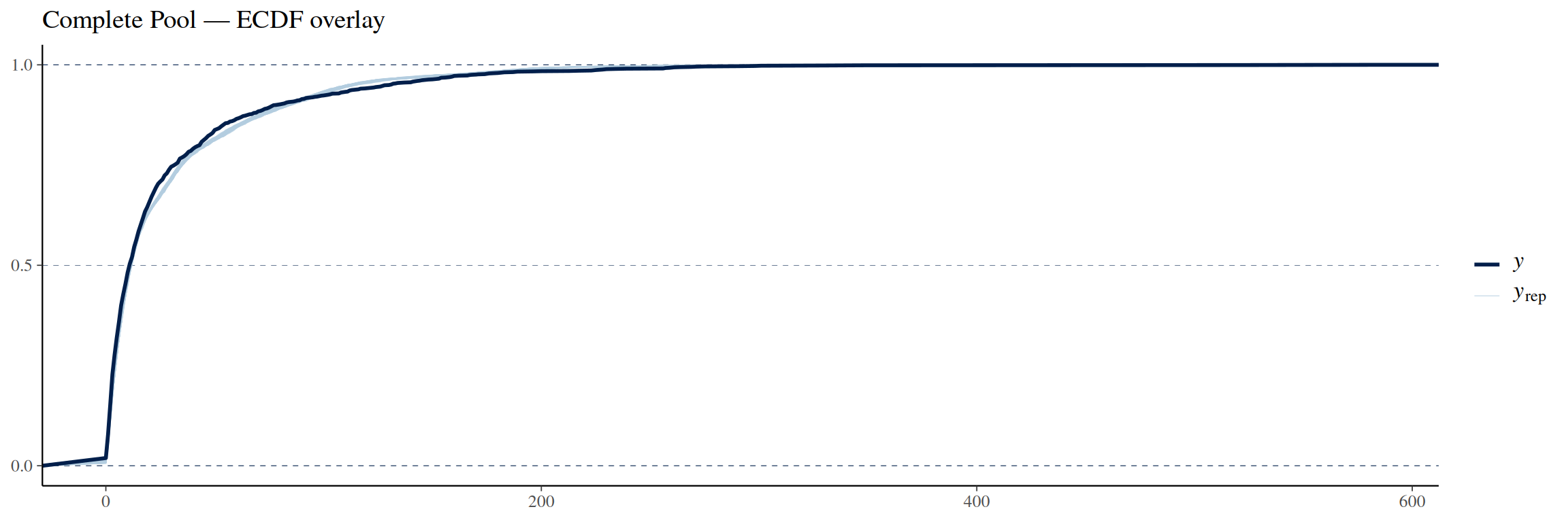
pp_check(complete_pool_model, ndraws = 100, type = "ecdf_overlay") +
  labs(title = "Complete Pool — ECDF overlay")

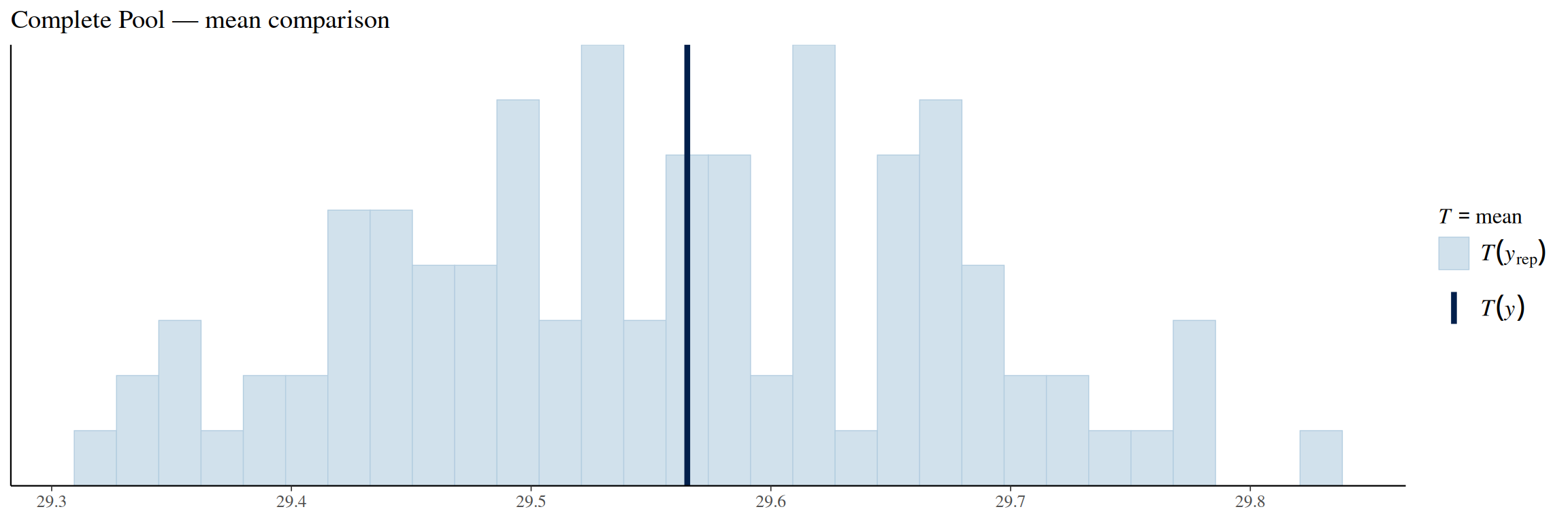
pp_check(complete_pool_model, ndraws = 100, type = "stat", stat = "mean") +
  labs(title = "Complete Pool — mean comparison")

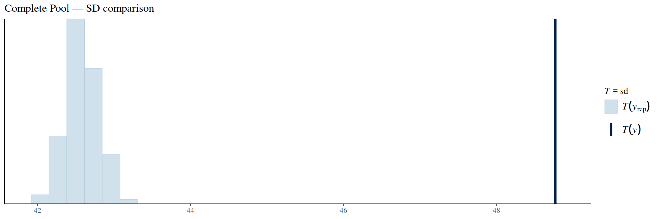
pp_check(complete_pool_model, ndraws = 100, type = "stat", stat = "sd") +
  labs(title = "Complete Pool — SD comparison")

The complete pooling model ECDF follows the observed ECDF better at low fatalities than the no pooling model, but it still struggles in the 25–100 fatalities region.

The mean comparison plot shows that the observed mean is almost at the exact center of the model simulated fatalities distribution, meaning that this model also estimates the overall fatality rate correctly.

The standard deviation comparison plot shows that this model is also under-dispersed, but the effect is smaller than with the no pooling model.

Predictions Over Time

pred_data <- tibble(
  year_scaled = seq(min(crashes_filtered$year_scaled),
                    max(crashes_filtered$year_scaled),
                    length.out = 100),
  aboard = round(mean(crashes_filtered$aboard))
)

predictions <- pred_data %>%
  add_epred_draws(complete_pool_model, ndraws = 1000) %>%
  mutate(.epred_rate = .epred / aboard)

ggplot() +
  stat_lineribbon(
    data = predictions,
    aes(x = year_scaled, y = .epred_rate),
    .width = c(0.50, 0.80, 0.95),
    alpha = 0.5
  ) +
  geom_point(
    data = crashes_filtered,
    aes(x = year_scaled, y = fatality_rate),
    alpha = 0.2,
    size = 1
  ) +
  scale_fill_brewer(palette = "Blues") +
  labs(
    title = "Complete Pooling Model: Fatality Rate Over Time",
    subtitle = paste0("Predictions for flights with ",
                     round(mean(crashes_filtered$aboard)), " people aboard (mean)"),
    x = "Year (Standardized)",
    y = "Fatality Rate",
    fill = "Credible Interval"
  )

Prior Sensitivity Analysis

We conduct a prior sensitivity analysis on this model by trying out 3 different prior settings and comparing the estimated parameters. The priors we are using are:

• Model prior: Intercept prior: \(\mathcal{N}(1.4, 1)\), year coefficient prior: \(\mathcal{N}(0, 0.5)\) (same as the model).
• Wide prior: Intercept prior: \(\mathcal{N}(1.4, 3)\), year coefficient prior: \(\mathcal{N}(0, 1.5)\) (3 times as wide for both).
• Shifted prior: Intercept prior: \(\mathcal{N}(3.4, 1)\), year coefficient prior: \(\mathcal{N}(2, 0.5)\) (both priors shifted by 2 to the right).

Prior Distribution	\(\alpha\)	\(\beta\)
Model prior	0.81	−0.18
Wide prior	0.81	−0.18
Shifted prior	0.81	−0.18

The parameters are identical for all three priors. From these results it can be concluded that the model is very insensitive to the prior choice.

No pooling (non-hierarchical model)

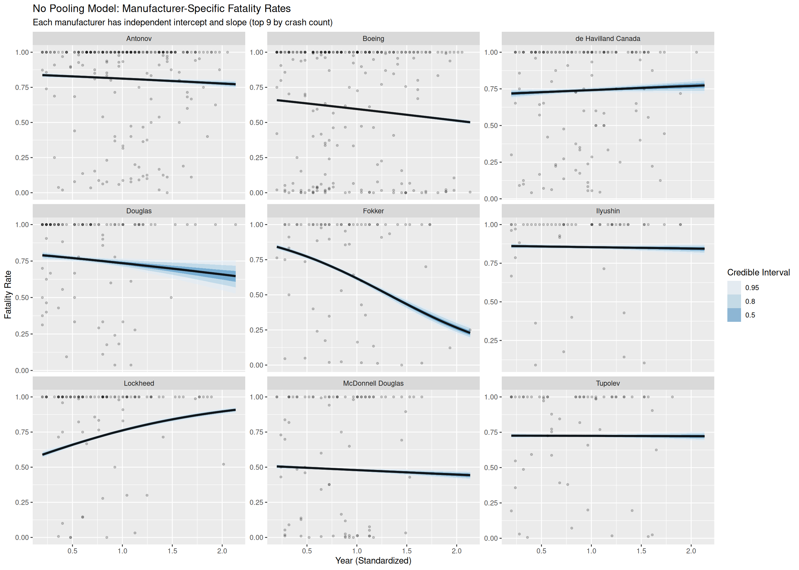
No Pooling Model

This model treats every airplane manufacturer as their own independent entity, without sharing any information across any other possible grouping in the data. With \(i\) being the index of a plane crash and \(m[i]\) being the manufacturer \(m\) for crash \(i\):

\[\begin{align*} \text{Likelihood:} \quad & \\ y_i &\sim \text{Binomial}(n_i, p_i) \\ \text{logit}(p_i) &= \alpha_{m[i]} + \beta_{m[i]} \cdot \text{year\_scaled}_i \\[1em] \text{Priors:} \quad & \\ \alpha_m &\sim \mathcal{N}(0,\, 1) \quad \text{for } m = 1, \ldots, M \\ \beta_m &\sim \mathcal{N}(0,\, 1) \quad \text{for } m = 1, \ldots, M \end{align*}\]

This means that the model assumes that each crash has its own fatality rate based on the manufacturer and the year, and crashes from other manufacturers do not influence each other in any way. With this model, the estimates for manufacturers with only a few crashes in the data become unstable, because they can’t borrow information from other manufacturers.

Model

no_pool_formula <- bf(
    fatalities | trials(aboard) ~ 0 + aircraft_manufacturer + aircraft_manufacturer:year_scaled,
    family = binomial(link = "logit")
    )

priors <- c(
        prior(normal(0, 1), class = b)
        )

no_pool_model <- brm(
    formula = no_pool_formula,
    prior = priors,
  data = crashes_filtered,
    seed = 42,
    refresh = 0,
    cores = 4,
    backend = "cmdstanr"
)

Running MCMC with 4 parallel chains...

Chain 4 finished in 18.2 seconds.
Chain 1 finished in 18.6 seconds.
Chain 2 finished in 19.7 seconds.
Chain 3 finished in 20.5 seconds.

All 4 chains finished successfully.
Mean chain execution time: 19.2 seconds.
Total execution time: 20.5 seconds.

Convergence Diagnostics

summary(no_pool_model)

 Family: binomial 
  Links: mu = logit 
Formula: fatalities | trials(aboard) ~ 0 + aircraft_manufacturer + aircraft_manufacturer:year_scaled 
   Data: crashes_filtered (Number of observations: 1766) 
  Draws: 4 chains, each with iter = 2000; warmup = 1000; thin = 1;
         total post-warmup draws = 4000

Regression Coefficients:
                                                   Estimate Est.Error l-95% CI
aircraft_manufacturerAerospatiale                      1.73      0.54     0.70
aircraft_manufacturerAirbus                            0.09      0.07    -0.05
aircraft_manufacturerAntonov                           1.68      0.08     1.52
aircraft_manufacturerATR                               0.35      0.42    -0.46
aircraft_manufacturerBeechcraft                        1.84      0.44     1.01
aircraft_manufacturerBell                              1.94      0.40     1.18
aircraft_manufacturerBoeing                            0.72      0.03     0.67
aircraft_manufacturerBritishAerospace                 -0.75      0.44    -1.60
aircraft_manufacturerBritten                           1.26      0.28     0.73
aircraft_manufacturerBrittenNorman                     0.72      0.37    -0.01
aircraft_manufacturerCanadair                          0.35      0.53    -0.68
aircraft_manufacturerCASA                              1.51      0.42     0.69
aircraft_manufacturerCASA212Aviocar                   -0.24      0.47    -1.16
aircraft_manufacturerCessna                            1.52      0.44     0.68
aircraft_manufacturerConvair                           0.90      0.22     0.48
aircraft_manufacturerDeHavilland                       1.75      0.30     1.17
aircraft_manufacturerdeHavillandCanada                 0.91      0.11     0.69
aircraft_manufacturerDornier                          -0.09      0.47    -0.99
aircraft_manufacturerDouglas                           1.40      0.11     1.17
aircraft_manufacturerEmbraer                           1.25      0.37     0.52
aircraft_manufacturerEmbraer110P1                      2.00      0.50     1.04
aircraft_manufacturerFairchild                         3.16      0.31     2.57
aircraft_manufacturerFokker                            1.97      0.10     1.77
aircraft_manufacturerGrumman                          -0.03      0.36    -0.71
aircraft_manufacturerHawkerSiddeley                    0.39      0.19     0.02
aircraft_manufacturerIlyushin                          1.84      0.10     1.64
aircraft_manufacturerLearjet                           1.31      0.66     0.04
aircraft_manufacturerLet                               0.09      0.40    -0.69
aircraft_manufacturerLockheed                          0.16      0.07     0.03
aircraft_manufacturerMcDonnellDouglas                  0.05      0.04    -0.04
aircraft_manufacturerMi                               -0.84      0.34    -1.51
aircraft_manufacturerMil                               4.33      0.36     3.64
aircraft_manufacturerPilatus                           1.05      0.60    -0.08
aircraft_manufacturerPiper                             1.61      0.39     0.87
aircraft_manufacturerShorts                           -0.25      0.39    -0.97
aircraft_manufacturerSikorsky                          0.77      0.21     0.37
aircraft_manufacturerSwearingen                        2.34      0.56     1.23
aircraft_manufacturerTupolev                           0.98      0.06     0.86
aircraft_manufacturerVickersViscount                   2.42      0.34     1.77
aircraft_manufacturerYakovlev                          0.60      0.15     0.29
aircraft_manufacturerAerospatiale:year_scaled         -0.14      0.54    -1.20
aircraft_manufacturerAirbus:year_scaled                0.04      0.05    -0.07
aircraft_manufacturerAntonov:year_scaled              -0.22      0.07    -0.36
aircraft_manufacturerATR:year_scaled                   0.55      0.25     0.06
aircraft_manufacturerBeechcraft:year_scaled            0.43      0.42    -0.38
aircraft_manufacturerBell:year_scaled                  0.81      0.46    -0.05
aircraft_manufacturerBoeing:year_scaled               -0.34      0.03    -0.39
aircraft_manufacturerBritishAerospace:year_scaled      1.32      0.47     0.41
aircraft_manufacturerBritten:year_scaled              -0.05      0.29    -0.63
aircraft_manufacturerBrittenNorman:year_scaled         0.32      0.37    -0.41
aircraft_manufacturerCanadair:year_scaled              0.66      0.37    -0.06
aircraft_manufacturerCASA:year_scaled                  0.16      0.36    -0.54
aircraft_manufacturerCASA212Aviocar:year_scaled        2.07      0.60     0.90
aircraft_manufacturerCessna:year_scaled               -0.75      0.47    -1.65
aircraft_manufacturerConvair:year_scaled              -0.65      0.26    -1.16
aircraft_manufacturerDeHavilland:year_scaled          -0.22      0.28    -0.77
aircraft_manufacturerdeHavillandCanada:year_scaled     0.15      0.11    -0.07
aircraft_manufacturerDornier:year_scaled               1.04      0.38     0.30
aircraft_manufacturerDouglas:year_scaled              -0.37      0.16    -0.69
aircraft_manufacturerEmbraer:year_scaled              -0.43      0.26    -0.95
aircraft_manufacturerEmbraer110P1:year_scaled         -0.17      0.61    -1.35
aircraft_manufacturerFairchild:year_scaled            -1.35      0.47    -2.24
aircraft_manufacturerFokker:year_scaled               -1.49      0.10    -1.69
aircraft_manufacturerGrumman:year_scaled               0.57      0.40    -0.22
aircraft_manufacturerHawkerSiddeley:year_scaled        0.03      0.26    -0.47
aircraft_manufacturerIlyushin:year_scaled             -0.07      0.10    -0.27
aircraft_manufacturerLearjet:year_scaled               0.71      0.59    -0.46
aircraft_manufacturerLet:year_scaled                   0.40      0.30    -0.20
aircraft_manufacturerLockheed:year_scaled              1.00      0.09     0.82
aircraft_manufacturerMcDonnellDouglas:year_scaled     -0.13      0.05    -0.24
aircraft_manufacturerMi:year_scaled                    1.86      0.29     1.30
aircraft_manufacturerMil:year_scaled                  -1.67      0.29    -2.25
aircraft_manufacturerPilatus:year_scaled               1.14      0.57     0.04
aircraft_manufacturerPiper:year_scaled                 0.12      0.44    -0.73
aircraft_manufacturerShorts:year_scaled                1.11      0.42     0.30
aircraft_manufacturerSikorsky:year_scaled              0.92      0.26     0.44
aircraft_manufacturerSwearingen:year_scaled           -0.73      0.42    -1.56
aircraft_manufacturerTupolev:year_scaled              -0.01      0.06    -0.13
aircraft_manufacturerVickersViscount:year_scaled       1.98      0.77     0.50
aircraft_manufacturerYakovlev:year_scaled              0.56      0.18     0.22
                                                   u-95% CI Rhat Bulk_ESS
aircraft_manufacturerAerospatiale                      2.81 1.00     4747
aircraft_manufacturerAirbus                            0.23 1.00     3881
aircraft_manufacturerAntonov                           1.84 1.00     4704
aircraft_manufacturerATR                               1.16 1.00     5518
aircraft_manufacturerBeechcraft                        2.72 1.00     4993
aircraft_manufacturerBell                              2.73 1.00     5577
aircraft_manufacturerBoeing                            0.78 1.00     5567
aircraft_manufacturerBritishAerospace                  0.10 1.00     5224
aircraft_manufacturerBritten                           1.82 1.00     4878
aircraft_manufacturerBrittenNorman                     1.47 1.00     5396
aircraft_manufacturerCanadair                          1.40 1.00     5786
aircraft_manufacturerCASA                              2.35 1.00     4962
aircraft_manufacturerCASA212Aviocar                    0.67 1.00     5992
aircraft_manufacturerCessna                            2.38 1.00     5434
aircraft_manufacturerConvair                           1.33 1.00     5522
aircraft_manufacturerDeHavilland                       2.35 1.00     5343
aircraft_manufacturerdeHavillandCanada                 1.12 1.00     5440
aircraft_manufacturerDornier                           0.79 1.00     4284
aircraft_manufacturerDouglas                           1.62 1.00     5141
aircraft_manufacturerEmbraer                           1.99 1.00     5328
aircraft_manufacturerEmbraer110P1                      2.96 1.00     5831
aircraft_manufacturerFairchild                         3.79 1.00     5244
aircraft_manufacturerFokker                            2.17 1.00     5480
aircraft_manufacturerGrumman                           0.66 1.00     5634
aircraft_manufacturerHawkerSiddeley                    0.76 1.00     5878
aircraft_manufacturerIlyushin                          2.04 1.00     4950
aircraft_manufacturerLearjet                           2.65 1.00     6256
aircraft_manufacturerLet                               0.86 1.00     5045
aircraft_manufacturerLockheed                          0.30 1.00     4761
aircraft_manufacturerMcDonnellDouglas                  0.14 1.00     5539
aircraft_manufacturerMi                               -0.18 1.00     5518
aircraft_manufacturerMil                               5.05 1.00     5616
aircraft_manufacturerPilatus                           2.24 1.00     4946
aircraft_manufacturerPiper                             2.38 1.00     5644
aircraft_manufacturerShorts                            0.51 1.00     5593
aircraft_manufacturerSikorsky                          1.18 1.00     5416
aircraft_manufacturerSwearingen                        3.48 1.00     5954
aircraft_manufacturerTupolev                           1.09 1.00     5624
aircraft_manufacturerVickersViscount                   3.09 1.00     5859
aircraft_manufacturerYakovlev                          0.89 1.00     5685
aircraft_manufacturerAerospatiale:year_scaled          0.89 1.00     4951
aircraft_manufacturerAirbus:year_scaled                0.15 1.00     4166
aircraft_manufacturerAntonov:year_scaled              -0.07 1.00     5404
aircraft_manufacturerATR:year_scaled                   1.04 1.00     5408
aircraft_manufacturerBeechcraft:year_scaled            1.26 1.00     4928
aircraft_manufacturerBell:year_scaled                  1.74 1.00     6039
aircraft_manufacturerBoeing:year_scaled               -0.29 1.00     5440
aircraft_manufacturerBritishAerospace:year_scaled      2.23 1.00     5331
aircraft_manufacturerBritten:year_scaled               0.54 1.00     5314
aircraft_manufacturerBrittenNorman:year_scaled         1.06 1.00     5063
aircraft_manufacturerCanadair:year_scaled              1.39 1.00     5781
aircraft_manufacturerCASA:year_scaled                  0.85 1.00     5074
aircraft_manufacturerCASA212Aviocar:year_scaled        3.23 1.00     5826
aircraft_manufacturerCessna:year_scaled                0.17 1.00     5634
aircraft_manufacturerConvair:year_scaled              -0.14 1.00     5428
aircraft_manufacturerDeHavilland:year_scaled           0.34 1.00     5086
aircraft_manufacturerdeHavillandCanada:year_scaled     0.37 1.00     5531
aircraft_manufacturerDornier:year_scaled               1.80 1.00     4129
aircraft_manufacturerDouglas:year_scaled              -0.05 1.00     5423
aircraft_manufacturerEmbraer:year_scaled               0.08 1.00     4936
aircraft_manufacturerEmbraer110P1:year_scaled          1.04 1.00     5619
aircraft_manufacturerFairchild:year_scaled            -0.42 1.00     5031
aircraft_manufacturerFokker:year_scaled               -1.29 1.00     5282
aircraft_manufacturerGrumman:year_scaled               1.36 1.00     6058
aircraft_manufacturerHawkerSiddeley:year_scaled        0.54 1.00     5739
aircraft_manufacturerIlyushin:year_scaled              0.13 1.00     4788
aircraft_manufacturerLearjet:year_scaled               1.91 1.00     5934
aircraft_manufacturerLet:year_scaled                   0.98 1.00     5059
aircraft_manufacturerLockheed:year_scaled              1.17 1.00     4957
aircraft_manufacturerMcDonnellDouglas:year_scaled     -0.02 1.00     5721
aircraft_manufacturerMi:year_scaled                    2.44 1.00     5605
aircraft_manufacturerMil:year_scaled                  -1.11 1.00     5617
aircraft_manufacturerPilatus:year_scaled               2.30 1.00     5110
aircraft_manufacturerPiper:year_scaled                 0.98 1.00     5638
aircraft_manufacturerShorts:year_scaled                1.93 1.00     5583
aircraft_manufacturerSikorsky:year_scaled              1.44 1.00     5156
aircraft_manufacturerSwearingen:year_scaled            0.11 1.00     5913
aircraft_manufacturerTupolev:year_scaled               0.11 1.00     5401
aircraft_manufacturerVickersViscount:year_scaled       3.53 1.00     5626
aircraft_manufacturerYakovlev:year_scaled              0.91 1.00     5735
                                                   Tail_ESS
aircraft_manufacturerAerospatiale                      2991
aircraft_manufacturerAirbus                            2926
aircraft_manufacturerAntonov                           2805
aircraft_manufacturerATR                               3004
aircraft_manufacturerBeechcraft                        3324
aircraft_manufacturerBell                              3170
aircraft_manufacturerBoeing                            3083
aircraft_manufacturerBritishAerospace                  2746
aircraft_manufacturerBritten                           2867
aircraft_manufacturerBrittenNorman                     3164
aircraft_manufacturerCanadair                          3206
aircraft_manufacturerCASA                              2969
aircraft_manufacturerCASA212Aviocar                    3059
aircraft_manufacturerCessna                            3051
aircraft_manufacturerConvair                           3111
aircraft_manufacturerDeHavilland                       2783
aircraft_manufacturerdeHavillandCanada                 2967
aircraft_manufacturerDornier                           2906
aircraft_manufacturerDouglas                           3272
aircraft_manufacturerEmbraer                           3078
aircraft_manufacturerEmbraer110P1                      2952
aircraft_manufacturerFairchild                         3118
aircraft_manufacturerFokker                            3266
aircraft_manufacturerGrumman                           3251
aircraft_manufacturerHawkerSiddeley                    2733
aircraft_manufacturerIlyushin                          3135
aircraft_manufacturerLearjet                           3306
aircraft_manufacturerLet                               2763
aircraft_manufacturerLockheed                          3228
aircraft_manufacturerMcDonnellDouglas                  3237
aircraft_manufacturerMi                                3143
aircraft_manufacturerMil                               2930
aircraft_manufacturerPilatus                           3247
aircraft_manufacturerPiper                             3292
aircraft_manufacturerShorts                            3105
aircraft_manufacturerSikorsky                          2763
aircraft_manufacturerSwearingen                        2962
aircraft_manufacturerTupolev                           2953
aircraft_manufacturerVickersViscount                   3294
aircraft_manufacturerYakovlev                          3064
aircraft_manufacturerAerospatiale:year_scaled          3102
aircraft_manufacturerAirbus:year_scaled                3087
aircraft_manufacturerAntonov:year_scaled               2808
aircraft_manufacturerATR:year_scaled                   2869
aircraft_manufacturerBeechcraft:year_scaled            3107
aircraft_manufacturerBell:year_scaled                  3417
aircraft_manufacturerBoeing:year_scaled                3197
aircraft_manufacturerBritishAerospace:year_scaled      2790
aircraft_manufacturerBritten:year_scaled               2815
aircraft_manufacturerBrittenNorman:year_scaled         2767
aircraft_manufacturerCanadair:year_scaled              3040
aircraft_manufacturerCASA:year_scaled                  3175
aircraft_manufacturerCASA212Aviocar:year_scaled        3061
aircraft_manufacturerCessna:year_scaled                3140
aircraft_manufacturerConvair:year_scaled               3274
aircraft_manufacturerDeHavilland:year_scaled           2595
aircraft_manufacturerdeHavillandCanada:year_scaled     3247
aircraft_manufacturerDornier:year_scaled               3014
aircraft_manufacturerDouglas:year_scaled               3312
aircraft_manufacturerEmbraer:year_scaled               2826
aircraft_manufacturerEmbraer110P1:year_scaled          2871
aircraft_manufacturerFairchild:year_scaled             3023
aircraft_manufacturerFokker:year_scaled                3212
aircraft_manufacturerGrumman:year_scaled               2922
aircraft_manufacturerHawkerSiddeley:year_scaled        2928
aircraft_manufacturerIlyushin:year_scaled              3217
aircraft_manufacturerLearjet:year_scaled               3209
aircraft_manufacturerLet:year_scaled                   2850
aircraft_manufacturerLockheed:year_scaled              3094
aircraft_manufacturerMcDonnellDouglas:year_scaled      3575
aircraft_manufacturerMi:year_scaled                    3147
aircraft_manufacturerMil:year_scaled                   3004
aircraft_manufacturerPilatus:year_scaled               3014
aircraft_manufacturerPiper:year_scaled                 2996
aircraft_manufacturerShorts:year_scaled                2927
aircraft_manufacturerSikorsky:year_scaled              3246
aircraft_manufacturerSwearingen:year_scaled            2995
aircraft_manufacturerTupolev:year_scaled               3304
aircraft_manufacturerVickersViscount:year_scaled       3293
aircraft_manufacturerYakovlev:year_scaled              2951

Draws were sampled using sample(hmc). For each parameter, Bulk_ESS
and Tail_ESS are effective sample size measures, and Rhat is the potential
scale reduction factor on split chains (at convergence, Rhat = 1).

The \(\hat{R}\) value for each of the parameters is 1.00, which means all coefficients converged properly. The bulk ESS values vary on the scale [4200, 5800] and the tail ESS values on the scale [2600, 3500]. These ESS values are far more than is needed for a reliable posterior estimation, so no problems there. The model had no divergences.

Posterior Predictive Check

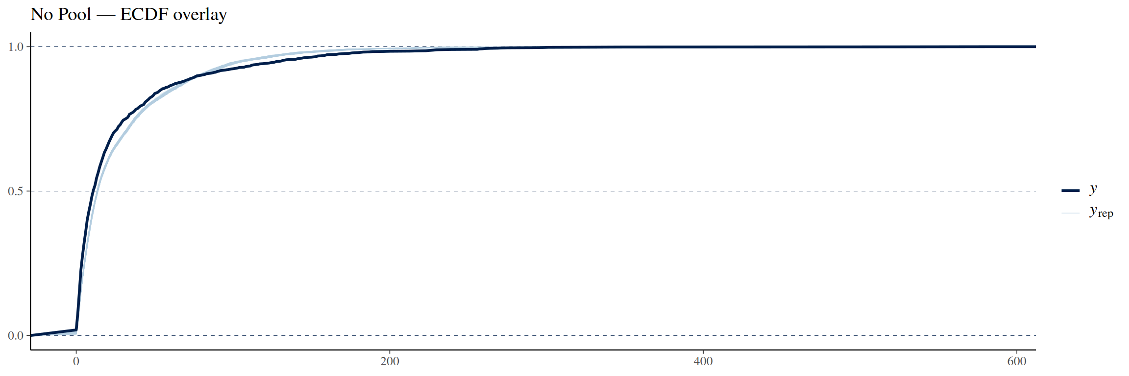
pp_check(no_pool_model, ndraws = 100, type = "ecdf_overlay") +
  labs(title = "No Pool — ECDF overlay")

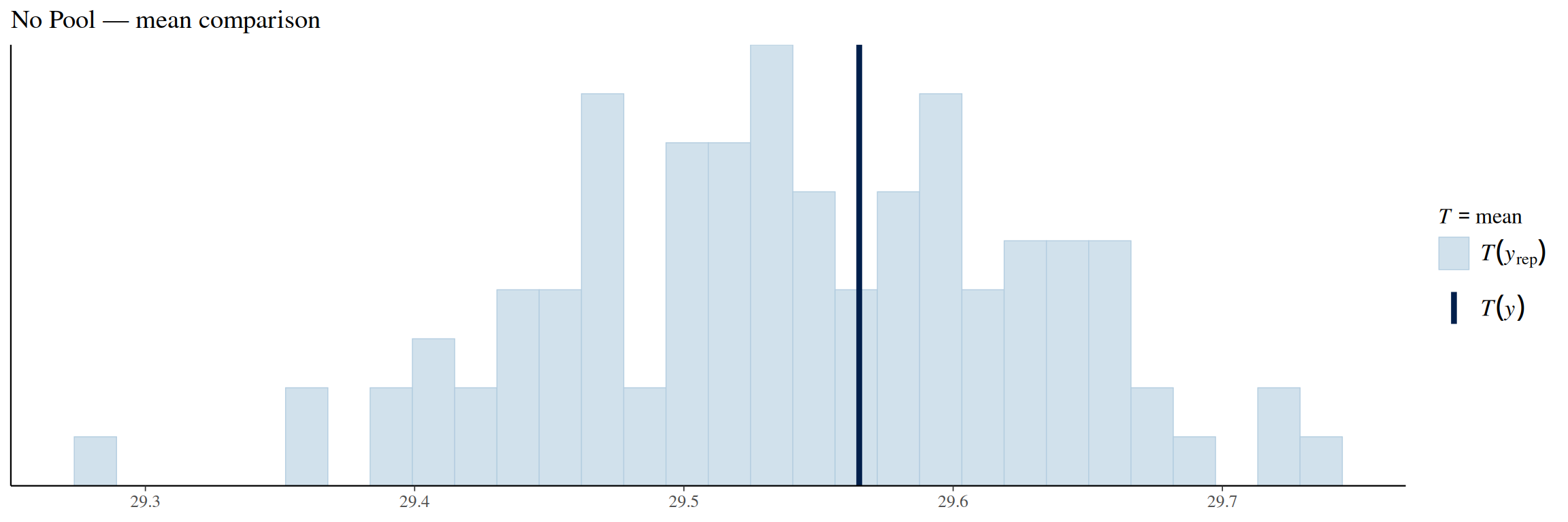
pp_check(no_pool_model, ndraws = 100, type = "stat", stat = "mean") +
  labs(title = "No Pool — mean comparison")

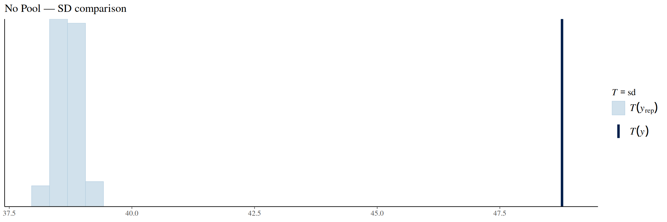
pp_check(no_pool_model, ndraws = 100, type = "stat", stat = "sd") +
  labs(title = "No Pool — SD comparison")

The ECDF (empirical cumulative distribution function) shows that the model is slightly off when compared to the real data. We can see that at the start, the observed ECDF rises faster and higher than the model ECDF, indicating that the model predicts less crashes with close to 0 fatalities. However, in the 25–100 fatalities area, the observed ECDF lags behind the model ECDF meaning that the model estimates more crashes that lead to those fatality numbers.

The mean comparison plot shows that the true fatalities mean lies close to the center of the model simulated fatalities distribution, meaning that the model estimates the overall mean fatality rate correctly.

The standard deviation comparison plot shows that the true fatalities standard deviation is much larger than what the model estimates. In other words, the model predicts too little variability and is under-dispersed.

Predictions by Manufacturer

top_manufacturers <- crashes_filtered %>%
  count(aircraft_manufacturer, sort = TRUE) %>%
  slice_head(n = 9) %>%
  pull(aircraft_manufacturer)

pred_data <- expand_grid(
  aircraft_manufacturer = top_manufacturers,
  year_scaled = seq(min(crashes_filtered$year_scaled),
                    max(crashes_filtered$year_scaled),
                    length.out = 100)
) %>%
  mutate(aboard = round(mean(crashes_filtered$aboard)))

predictions <- pred_data %>%
  add_epred_draws(no_pool_model, ndraws = 1000) %>%
  mutate(.epred_rate = .epred / aboard)

ggplot() +
  stat_lineribbon(
    data = predictions,
    aes(x = year_scaled, y = .epred_rate),
    .width = c(0.50, 0.80, 0.95),
    alpha = 0.5
  ) +
  geom_point(
    data = crashes_filtered %>% filter(aircraft_manufacturer %in% top_manufacturers),
    aes(x = year_scaled, y = fatality_rate),
    alpha = 0.2,
    size = 1
  ) +
  facet_wrap(~ aircraft_manufacturer, scales = "free_y", ncol = 3) +
  scale_fill_brewer(palette = "Blues") +
  labs(
    title = "No Pooling Model: Manufacturer-Specific Fatality Rates",
    subtitle = "Each manufacturer has independent intercept and slope (top 9 by crash count)",
    x = "Year (Standardized)",
    y = "Fatality Rate",
    fill = "Credible Interval"
  )

Prior Sensitivity Analysis

We conduct a prior sensitivity analysis on this model by trying out 3 different priors and comparing the estimated parameters of 4 manufacturers. The priors we are using are:

• Model prior: \(\mathcal{N}(0, 1)\) (same as the model).
• Wide prior: \(\mathcal{N}(0, 3)\) (a much wider distribution).
• Shifted prior: \(\mathcal{N}(2, 1)\) (shifted to the right).

Prior Distribution	Manufacturer	\(\alpha\)	\(\beta\)
Model \(\mathcal{N}(0, 1)\)	Boeing	0.72	−0.34
	Bell	1.94	0.82
	Lockheed	0.16	1.00
	Mil	4.34	−1.67
Wide \(\mathcal{N}(0, 3)\)	Boeing	0.72	−0.34
	Bell	2.20	0.63
	Lockheed	0.16	1.00
	Mil	5.16	−2.30
Shifted \(\mathcal{N}(2, 1)\)	Boeing	0.72	−0.34
	Bell	1.96	0.96
	Lockheed	0.16	1.00
	Mil	4.40	−1.70

We can see that the parameters do not vary much. For manufacturers with many observations in the data (Boeing: 248 observations, Lockheed: 106 observations), the parameters are identical for every prior. For manufacturers with a fewer number of observations (Mil: 41 observations, Bell: 33 observations), the parameter values show more variance:

\[\text{Mil: } \operatorname{Var}(\alpha) \approx 0.21,\quad \operatorname{Var}(\beta) \approx 0.11\] \[\text{Bell: } \operatorname{Var}(\alpha) \approx 0.02,\quad \operatorname{Var}(\beta) \approx 0.03\]

These variances are tolerable and still show the same trend, just in different strengths. The results show that the model is stable under reasonable prior changes, and the main conclusions drawn from the model do not depend on the chosen prior.

Partial pooling (hierarchical model)

Partial Pooling Model

For the partially pooled model, we are predicting both a population level intercept and coefficient (\(\alpha_0\) and \(\beta_0\)) and manufacturer level intercepts and coefficients (\(\alpha_{m[i]}\) and \(\beta_{m[i]}\)). The partial pooling model is a combination of the techniques used in the no pooling model and the complete pooling model. The no pooling method assumed that each manufacturer had their own intercept and coefficient and the complete pooling model assumed that all manufacturers have the same intercept and coefficient. The partial pooling assumes that both of these conditions hold.

\[\begin{align*} \text{Likelihood:} \quad & \\ y_i &\sim \text{Binomial}(n_i, p_i) \\ \text{logit}(p_i) &= \alpha_0 + \beta_0 \cdot \text{year\_scaled}_i + \alpha_{m[i]} + \beta_{m[i]} \cdot \text{year\_scaled}_i \\[1em] \text{Random effects:} \quad & \\ \begin{bmatrix} \alpha_m \\ \beta_m \end{bmatrix} &\sim \mathcal{N}\!\left(\begin{bmatrix} 0 \\ 0 \end{bmatrix},\, \boldsymbol{\Sigma}\right), \quad \boldsymbol{\Sigma} = \begin{bmatrix} \sigma_\alpha^2 & \rho\,\sigma_\alpha\sigma_\beta \\ \rho\,\sigma_\alpha\sigma_\beta & \sigma_\beta^2 \end{bmatrix} \\[1em] \text{Priors:} \quad & \\ \alpha_0 &\sim \mathcal{N}(1.4,\, 1) \\ \beta_0 &\sim \mathcal{N}(0,\, 0.5) \\ \sigma_\alpha,\, \sigma_\beta &\sim \mathcal{N}^+(0,\, 0.6) \\ \rho &\sim \text{LKJ}(2) \end{align*}\]

Model

hierarchical_formula <- bf(
  fatalities | trials(aboard) ~ 1 + year_scaled + (1 + year_scaled | aircraft_manufacturer),
  family = binomial(link = "logit")
  )

priors <- c(
    prior(normal(1.4, 1), class = Intercept),
    prior(normal(0, 0.5), class = b),
    prior(normal(0, 0.6), class = sd),
    prior(lkj(2), class = cor)
  )

partial_pool_model <- brm(
  formula = hierarchical_formula,
  prior = priors,
  data = crashes_filtered,
  seed = 42,
  control = list(adapt_delta = 0.95),
  refresh = 0,
  cores = 4,
  backend = "cmdstanr"
)

Running MCMC with 4 parallel chains...

Chain 4 finished in 71.4 seconds.
Chain 2 finished in 73.1 seconds.
Chain 3 finished in 80.4 seconds.
Chain 1 finished in 91.2 seconds.

All 4 chains finished successfully.
Mean chain execution time: 79.0 seconds.
Total execution time: 91.3 seconds.

Convergence Diagnostics

summary(partial_pool_model)

 Family: binomial 
  Links: mu = logit 
Formula: fatalities | trials(aboard) ~ 1 + year_scaled + (1 + year_scaled | aircraft_manufacturer) 
   Data: crashes_filtered (Number of observations: 1766) 
  Draws: 4 chains, each with iter = 2000; warmup = 1000; thin = 1;
         total post-warmup draws = 4000

Multilevel Hyperparameters:
~aircraft_manufacturer (Number of levels: 40) 
                           Estimate Est.Error l-95% CI u-95% CI Rhat Bulk_ESS
sd(Intercept)                  1.22      0.14     0.97     1.51 1.00     1189
sd(year_scaled)                0.92      0.12     0.71     1.15 1.01      824
cor(Intercept,year_scaled)    -0.75      0.08    -0.87    -0.56 1.00     1013
                           Tail_ESS
sd(Intercept)                  2115
sd(year_scaled)                1529
cor(Intercept,year_scaled)     1649

Regression Coefficients:
            Estimate Est.Error l-95% CI u-95% CI Rhat Bulk_ESS Tail_ESS
Intercept       1.27      0.20     0.88     1.66 1.00      441      971
year_scaled     0.02      0.15    -0.28     0.32 1.00      458     1138

Draws were sampled using sample(hmc). For each parameter, Bulk_ESS
and Tail_ESS are effective sample size measures, and Rhat is the potential
scale reduction factor on split chains (at convergence, Rhat = 1).

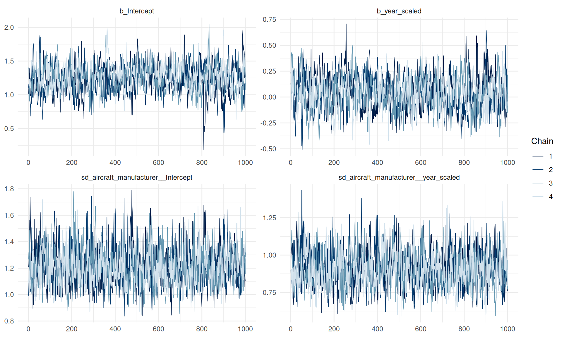
mcmc_plot(partial_pool_model, type = "trace",
          variable = c("b_Intercept", "b_year_scaled",
                      "sd_aircraft_manufacturer__Intercept",
                      "sd_aircraft_manufacturer__year_scaled"))

The partial pooling model MCMC converged well with all \(\hat{R}\) values smaller or equal to 1.01:

Parameter	\(\hat{R}\)	Bulk ESS	Tail ESS
\(\sigma_\alpha\) (SD Intercept)	1.00	875	1707
\(\sigma_\beta\) (SD year_scaled)	1.01	779	1184
\(\rho\) (Correlation)	1.00	961	1537
\(\alpha_0\) (Intercept)	1.01	511	959
\(\beta_0\) (year_scaled)	1.00	516	951

Even though our process converged, the low ESS values are troublesome. Both bulk ESS and tail ESS values should be over 1000 in an ideal case. The models ESS values are relatively close to 1000 for the standard deviation and correlation parameters, but are far away from ideal for the intercept \(\alpha_0\) and the coefficient \(\beta_0\). We tried doubling the warmup and iteration counts to 1000 and 4000 respectively, but the ESS numbers stay the same. This means that especially for \(\alpha_0\) and \(\beta_0\), we don’t have enough independent samples for truly reliable posterior estimates.

Posterior Predictive Check

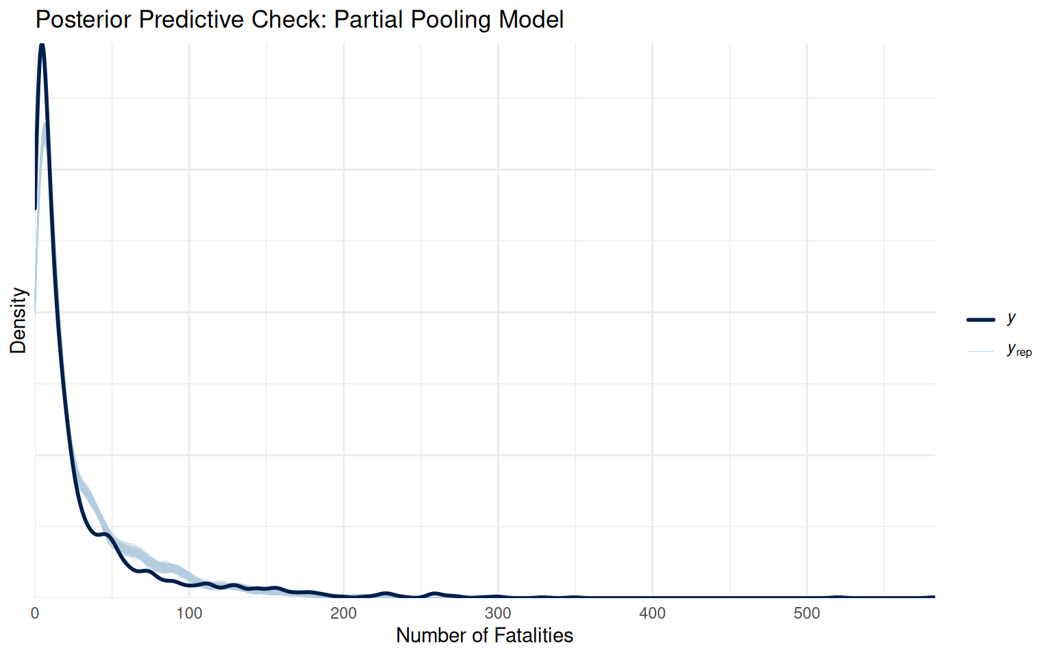
pp_check(partial_pool_model, ndraws = 100, type = "ecdf_overlay") +
  labs(title = "Partial Pool — ECDF overlay")

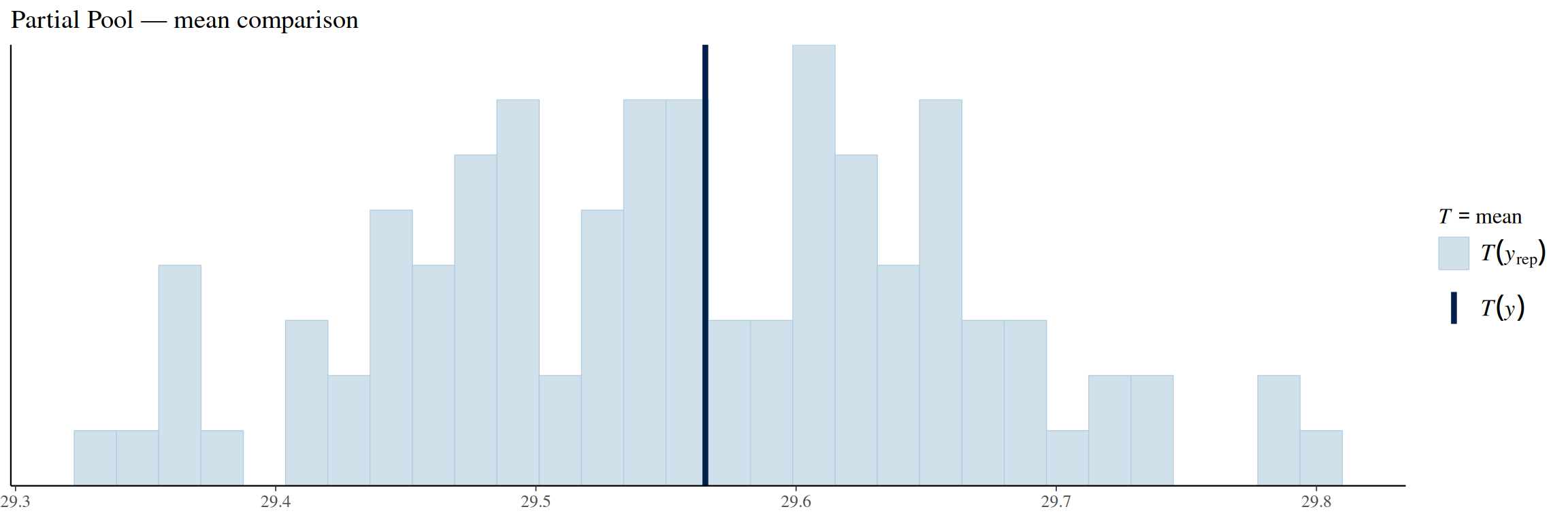
pp_check(partial_pool_model, ndraws = 100, type = "stat", stat = "mean") +
  labs(title = "Partial Pool — mean comparison")

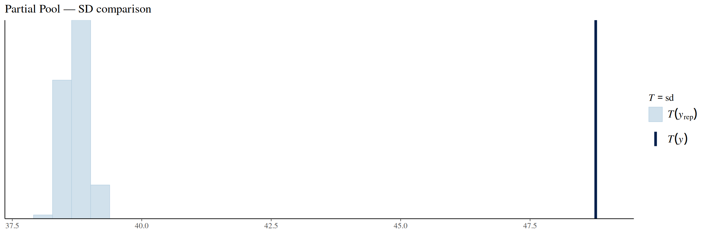
pp_check(partial_pool_model, ndraws = 100, type = "stat", stat = "sd") +
  labs(title = "Partial Pool — SD comparison")

The ECDF of the partially pooled model matches the original observations fairly well. Same for the observed mean. The standard deviation comparison has the same problem as the other two models: it is under-dispersed.

Prior Sensitivity Analysis

For the partial pooling model, we analyse how changing our prior assumptions on how similar manufacturers are affects the posterior predictions. We do this by using three different priors for our standard deviations \(\sigma\):

• Baseline: \(\sigma \sim \mathcal{N}^+(0, 0.6)\) (original)
• Tight: \(\sigma \sim \mathcal{N}^+(0, 0.3)\) (assumes manufacturers more similar)
• Wide: \(\sigma \sim \mathcal{N}^+(0, 1.2)\) (assumes manufacturers differ more)

Prior Scenario	Intercept Mean	Year Effect Mean	SD Manufacturer Mean
Baseline	1.271	0.019	1.205
Tight	1.263	0.024	1.037
Wide	1.280	0.016	1.295

The means don’t show noticeable effects from different prior choices. The standard deviation is affected by changing the prior distributions for it, but this is expected — the standard deviation priors should only affect the standard deviation posteriors. Thus we can conclude that our model is robust.

Model comparison

To compare the three models, we use LOO-CV (Leave-One-Out Cross-Validation), which has the basic idea of: 1) remove an observation \(i\), 2) train the model, 3) predict observation \(i\). Then measure how well the model performed and compare the models. We measure the ELPD (Expected Log Predictive Density) and SE (Standard Error) for all models and then compare them with each other. We use the partial pooling model as the baseline.

no_pool_loo <- loo(no_pool_model)
complete_pool_loo <- loo(complete_pool_model)
partial_pool_loo <- loo(partial_pool_model)

loo_compare(no_pool_loo, complete_pool_loo, partial_pool_loo)

                    elpd_diff se_diff
no_pool_model           0.0       0.0
partial_pool_model    -27.6      14.0
complete_pool_model -1974.0     691.8

Model	elpd_diff	se_diff	\(\lvert\text{elpd\_diff} / \text{se\_diff}\rvert\)
partial_pool_model	0.0	0.0	—
no_pool_model	−16.5	13.3	1.24
complete_pool_model	−1944.8	692.3	2.81

A good rule of thumb is that if \(|\text{elpd\_diff}| < 1 \times \text{se\_diff}\), the models are close to equal, and if \(|\text{elpd\_diff}| > 2 \times \text{se\_diff}\), there is a clear difference between the models. A higher ELPD value indicates better performance.

The no pooling model seems to perform slightly worse than the partial pooling model, but the ratio of 1.24 is still close to 1 and could just be due to random noise, so no clear conclusions can be drawn from this.

The complete pooling model, however, can be reported to perform significantly worse than the other two models. The reason for this is most likely that the model fails to capture the manufacturer level differences, and therefore predicts incorrectly for most crashes.

Discussion

Although the partial pooling model performs best according to LOO cross-validation, none of the three models succeeds in accurately modeling the structure of the real data, as revealed by the posterior predictive check analysis.

The two non-hierarchical models have their obvious limitations, but the interesting question is: why does the hierarchical model fail? On paper, it should perform well, because it uses population level information as well as captures the manufacturer level differences. Evidently, it still has its limitations.

The problem with all of our models seemed to be that they were under-dispersed, meaning that they underestimated the variance. The reason for this mainly comes from our use of binomial likelihood for predicting the fatalities. The variance formula of binomial likelihood for an observation \(i\) is

\[\operatorname{Var}(Y_i) = n_i p_i (1 - p_i)\]

This formula is fixed once \(n_i\) and \(p_i\) are known and is bounded by \(n_i / 4\) (when \(p_i = 0.5\)). The true variances in the observed data were shown to be much larger than the models’, because the binomial variance simply cannot reach the true variability values. As a potential improvement for the models, a different likelihood function that could combat this under-dispersion problem should be used.

Another reason that our models fail is much simpler. Airplane crashes simply cannot be modeled accurately, especially with so little information. There are countless factors that can affect the fatality rate of a crash and there is a lot of randomness included. One could try to add more predictors and see if it yields better results. But even with more predictors included, the results would still most likely be inaccurate, but perhaps better than what we reached.

Conclusions

In our report, we modeled fatality rate trends with hierarchical and non-hierarchical models. We used three types of models: complete pooling, no pooling and partial pooling models. From these models the partial pooling model performed the best with the no pooling model coming in a close second. We used LOO-CV to compare our models.

One of our research questions was whether there are differences in the fatality rates of manufacturers. The fact that the partial pooling and no pooling models performed well would suggest that fatalities are modeled better assuming that each manufacturer has their own parameters and distributions.

According to our prior sensitivity analysis, the models were quite unaffected by changes in priors. This means that our models are able to model the fatality rates well without the priors having too big of an effect on the model.

In our posterior predictive analysis, we noticed that our models weren’t capturing the variance of the original observations. The variance of our models was too small. This was due to the fixed maximum variance of the binomial model being too small to correctly model the real crash variance.

Self Reflection

The project was a great summary of the key concepts taught in the Bayesian Data Analysis course. During the course we acquired basic skills in Bayesian data analysis and during the project we got to use them in practice and deepen our understanding about the methods.

In this report we discussed things like hierarchical and non-hierarchical models, how to choose priors and test the effects of these priors on the predictions, how to run MCMC simulations and how to compare and evaluate the models these simulations suggest.

Running MCMC simulations is computationally expensive and the project showed the importance of access to cloud computing resources. Running the MCMC code could take over 30 minutes on old hardware while it took 5–10 minutes to run on modern cloud hardware in JupyterHub.

References

[1]

Jogwums, “Air crashes full data (1908-2024).” Kaggle, 2024. Available: https://www.kaggle.com/datasets/jogwums/air-crashes-full-data-1908-2023

[2]

Airways Magazine, “The history of commercial flight: How global travel took off,” Airways Magazine, Available: https://www.airwaysmag.com/legacy-posts/how-global-travel-took-off

[3]

Allianz Global Corporate & Specialty, “How aviation safety has improved,” 2015, Available: https://commercial.allianz.com/news-and-insights/expert-risk-articles/how-aviation-safety-has-improved.html